Omega group pay discrimination

Loading the data

We were provided with 50 records of data regarding salary, gender and number of years of experience.

omega <- read_csv(here::here("data", "omega.csv"))
glimpse(omega) 

## Rows: 50
## Columns: 3
## $ salary     <dbl> 81894, 69517, 68589, 74881, 65598, 76840, 78800, 70033, 635…
## $ gender     <chr> "male", "male", "male", "male", "male", "male", "male", "ma…
## $ experience <dbl> 16, 25, 15, 33, 16, 19, 32, 34, 1, 44, 7, 14, 33, 19, 24, 3…

Summary statistics

We can determine if women executives are discriminated by the company by analysing summary statistics on salary by gender.

mosaic::favstats (salary ~ gender, data=omega)

##   gender   min    Q1 median    Q3   max  mean   sd  n missing
## 1 female 47033 60338  64618 70033 78800 64543 7567 26       0
## 2   male 54768 68331  74675 78568 84576 73239 7463 24       0

formula_ci <-mosaic::favstats (salary ~ gender, data=omega) 
formula_ci %>% 
mutate(t_critical = qt(0.975,n-1),
       SE = sd/sqrt(n),
       margin_of_error = t_critical*sd,
       low_endpoint  = mean - margin_of_error,
       high_endpoint = mean + margin_of_error)

##   gender   min    Q1 median    Q3   max  mean   sd  n missing t_critical   SE
## 1 female 47033 60338  64618 70033 78800 64543 7567 26       0       2.06 1484
## 2   male 54768 68331  74675 78568 84576 73239 7463 24       0       2.07 1523
##   margin_of_error low_endpoint high_endpoint
## 1           15585        48958         80128
## 2           15438        57802         88677

Based on the confidence interval analysis as above, because the t statistic is larger than the critical value 1.96 for 95% confidence interval, we should reject the null hypothesis and conclude that there is a significant difference between the salaries of the male and female executives.

Hypothesis testing

Now, let’s try to analyse the issue at Omega Group by running a hypothesis testing using t.test function. We will assume that a null hypothesis means that, on average, men and women make the same amount of money.

# hypothesis testing using t.test() 
t.test(salary ~ gender, data = omega)

## 
##  Welch Two Sample t-test
## 
## data:  salary by gender
## t = -4, df = 48, p-value = 2e-04
## alternative hypothesis: true difference in means between group female and group male is not equal to 0
## 95 percent confidence interval:
##  -12973  -4420
## sample estimates:
## mean in group female   mean in group male 
##                64543                73239

This hypothesis test supports our previous findings. The p-value shown is very low, orders of magnitude below 0.05, which gives us enough support to reject the null hypothesis. This is further supported by the confidence intervals, which don’t include zero.

We can also use infer package to test our hypothesis whether women executives are indeed discriminated in Omega Group.

set.seed(3007)

omega_obs_diff <- omega %>%
  specify(response = salary, explanatory = gender) %>%
  hypothesise(null="independence") %>% 
  generate(reps = 1000, type = "permute") %>% 
  calculate(stat = "diff in means")

obs_mean <- omega %>%
  specify(response = salary, explanatory = gender) %>%
  calculate(stat = "diff in means")

omega_obs_diff %>% 
  visualise() +
  shade_p_value(obs_stat = obs_mean, direction = "two-sided")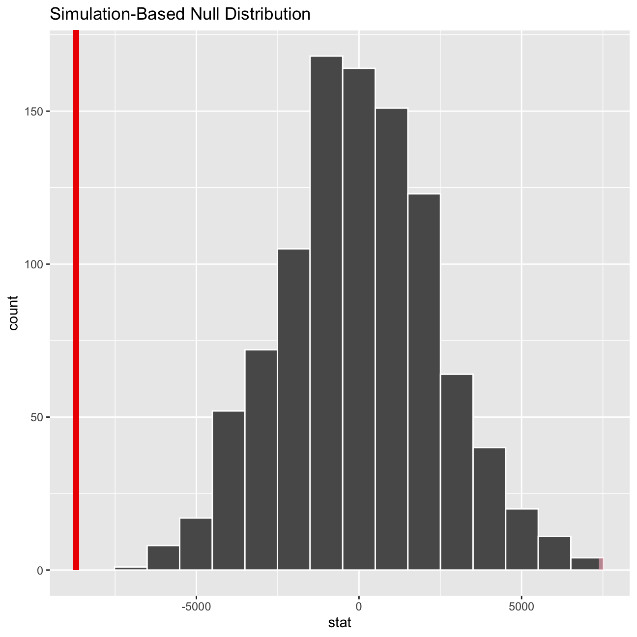

The infer package simulation supports the previous findings of the t.test and summary statistics. The observed mean falls very far away from the null distribution, so again we can reject the null hypothesis and conclude that there is strong evidence within the data set that gender has an impact in the salary of employees of Omega. There is a strong statistical difference between male salaries and female salaries, males earn on average 8696 units of currency more than their female counterparts.

Experience of male and female executives

Salary may also be influenced by the length of executive’s experience. Therefore, before we make a statement that female executives are subject to discrimination in Omega Group, we can inspect if male executives have significantly more experience than their female counterparts.

favstats (experience ~ gender, data=omega)

##   gender min    Q1 median   Q3 max  mean    sd  n missing
## 1 female   0  0.25    3.0 14.0  29  7.38  8.51 26       0
## 2   male   1 15.75   19.5 31.2  44 21.12 10.92 24       0

formula_ci <-mosaic::favstats (experience ~ gender, data=omega) 
formula_ci %>% 
mutate(t_critical = qt(0.975,n-1),
       SE = sd/sqrt(n),
       margin_of_error = t_critical*sd,
       low_endpoint  = mean - margin_of_error,
       high_endpoint = mean + margin_of_error)

##   gender min    Q1 median   Q3 max  mean    sd  n missing t_critical   SE
## 1 female   0  0.25    3.0 14.0  29  7.38  8.51 26       0       2.06 1.67
## 2   male   1 15.75   19.5 31.2  44 21.12 10.92 24       0       2.07 2.23
##   margin_of_error low_endpoint high_endpoint
## 1            17.5       -10.15          24.9
## 2            22.6        -1.46          43.7

Based on the confidence interval analysis as above, because the t-statistic is larger than the critical value 1.96 for 95% confidence interval, we should reject the null hypothesis and conclude that there is a significant difference between the experience of the male and female executives. Therefore, it could be the case that differences in experience between female and male contribute to difference in male and female salaries. The analysis here validates my conclusion about the difference in male and female salaries but we need to see the relationship between experience and salary.

Relationship between salary and experience

Finally, we can check if salary is correlated with experience. In order to do this, we will draw a scatter plot to visually inspect the relationship between salary and length of experience by gender.

omega %>% 
  ggplot(aes(x = salary, y = experience, color=gender)) +
  geom_smooth(method = "lm", fill="grey90", size=4) + 
  geom_point(size=2) +
  theme_minimal() +
  labs(
    title = "Relationship between Salary and Experience, by Gender",
    subtitle = "Omega Salary Dataset",
    caption = "Omega Group plc- Pay Discrimination",
    x = "Salary", y = "Experience"
  )+ 
  coord_flip()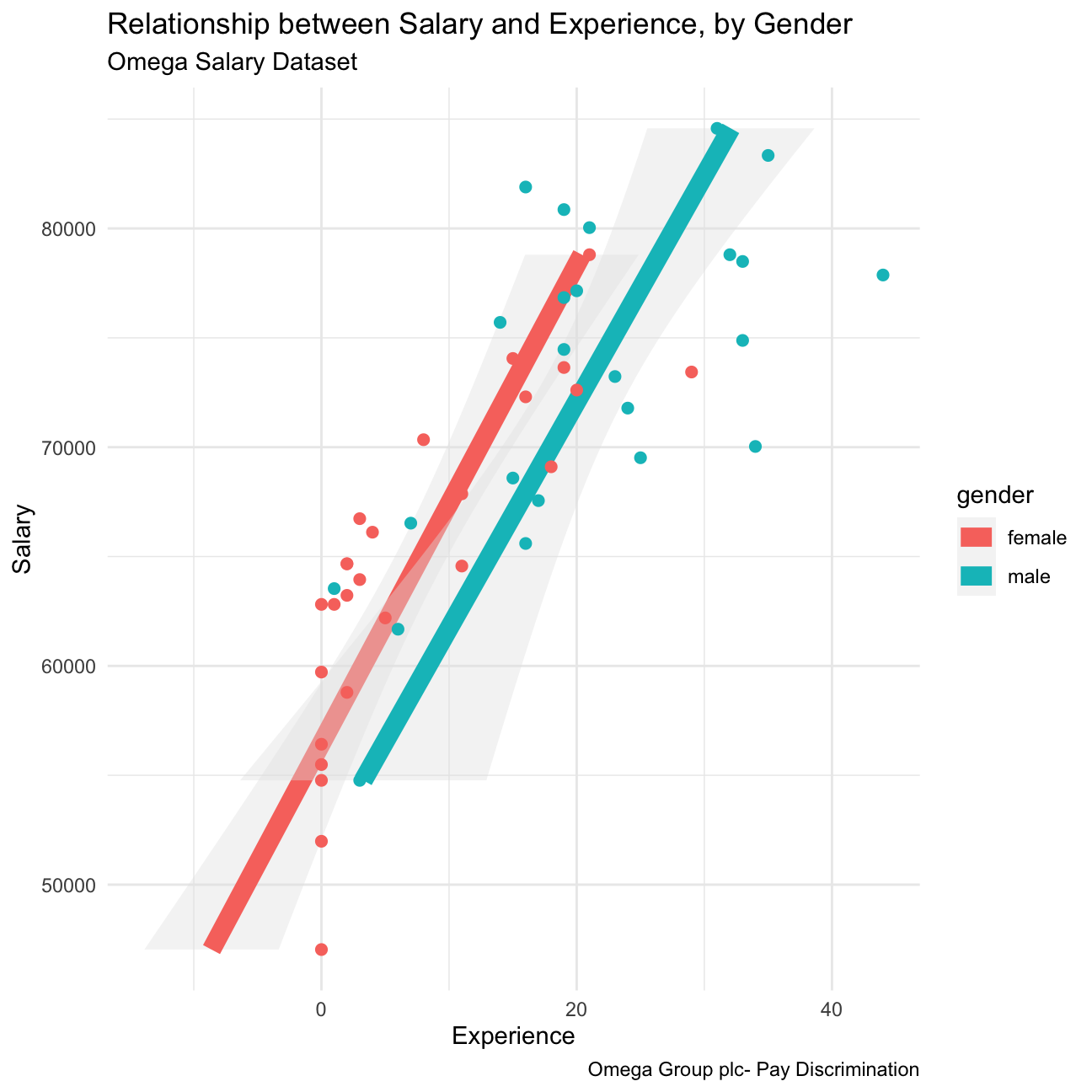

Correlations between gender, experience and salary

Now we can create a scatter plot and correlation matrix to determine the relationships between three variables: gender, experience and salary using ggpairs.

omega %>% 
  select(gender, experience, salary) %>% 
  ggpairs(aes(colour=gender, alpha = 0.3))+
  theme_bw()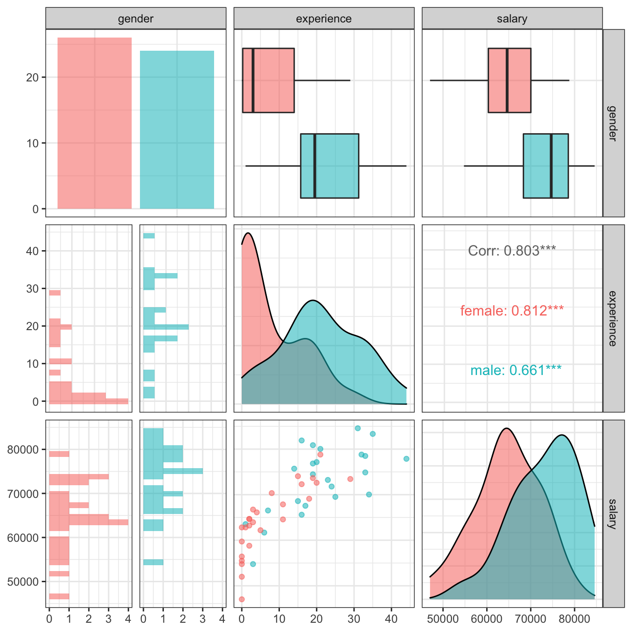

From the graph we can see that although average salary is greater for male executives than for female counterparts, women have on average significantly less experience than men. Looking at the distribution of experience it is clear that most of the female executives are quite junior in comparison to male executives. We can also spot a correlation between experience and salary, meaning that more experienced executives earn more on average irregardless of gender. Therefore, I believe there is no grounds to conclude that women executives are discriminated in Omega Group.